Business task

This analysis explores the relationship between Costa Rica’s exchange rate, interest rate differentials, and tourism arrivals to determine the optimal timing for purchasing CRC. Using correlation analysis and Granger Causality Tests on data from BCCR, ICT, and FRED, the goal is to help investors and bankers better understand how key economic variables influence exchange rate behavior and enhance their decision-making strategies.

Data sources used

The analysis uses publicly available, credible data from official sources:

• BCCR exchange rate and interest rate datasets
• ICT tourism arrivals dataset
• FRED Federal Funds Effective Rate dataset

The data covers the period from January 1, 2009 to December 31, 2024, organized daily or monthly depending on the source. To ensure consistency, monthly averages were calculated where necessary. All datasets were reviewed and show no missing values. There are no concerns regarding bias, licensing, privacy, or security. These datasets support robust correlation and causality analyses to evaluate the drivers of Costa Rica’s exchange rate.

Manipulation of data

Monthly averages were calculated from BCCR datasets using the formula:

=AVERAGEIFS(B6:B371, A6:A371, “*Ene*”, B6:B371, “>0”)

This method excludes zero values typically recorded on weekends or holidays, ensuring that averages reflect active market data only.

Analysis

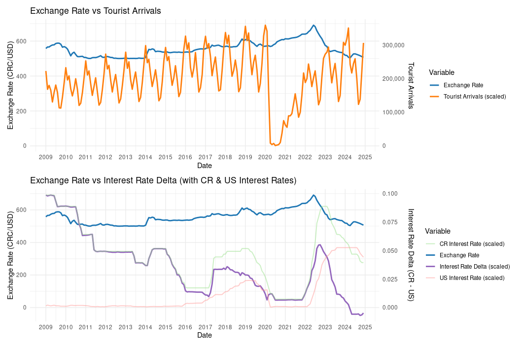
Tourist arrivals peak in January and drop in September. Major economic events—such as the 2008 U.S. financial crisis, 2014 BCCR policy shifts, 2018 fiscal crisis, and 2020 COVID-19 pandemic—corresponded with sharp exchange rate increases, followed by gradual normalization.

Despite a steady rise in tourism revenue, it has not significantly suppressed the exchange rate, with recent data showing increased tourism alongside a declining exchange rate. Interest rate differentials (CR – US) often rise after exchange rate shocks, suggesting a monetary policy response to attract capital inflows. However, the current historically low differential, paired with a continued decline in the exchange rate, casts doubt on the short-term predictive power of this metric.

These patterns indicate that neither tourism nor interest rate differentials alone can reliably forecast exchange rate trends, highlighting the need for a more integrated modeling approach when advising on CRC purchasing decisions.

Granger Causality Test Results:

• Tourist Arrivals → Exchange Rate: No significant causality (p = 0.1457 at 1 lag).
• Exchange Rate → Tourist Arrivals: Some reverse causality (p = 0.0839 at 4 lags), suggesting the exchange rate may influence tourism demand.
• Interest Rate Delta (CR – US) → Exchange Rate: Statistically significant (p = 0.0046), indicating the differential impacts the exchange rate.
• Exchange Rate → Interest Rate Delta: Strong reverse causality (p = 7.1e-06), suggesting exchange rate changes trigger monetary policy responses.
• Costa Rica’s Interest Rate → Exchange Rate: Very strong causality (p = 3.4e-08), showing a direct effect of domestic monetary policy on the exchange rate.

Visualizations

Further exploration

• Areas for deeper analysis include:
  • Capital inflows from international loans
  • Unrecorded currency inflows (e.g., narco dollars)
• Scenario analysis tools to simulate interest rate shocks and their effects on exchange rate dynamics.

Insights

• Domestic interest rates are the primary driver of Costa Rica’s exchange rate. Granger tests show strong causality and feedback effects, indicating that monetary policy both influences and responds to exchange rate changes.
• Tourism has limited influence on exchange rate movements. While some weak reverse causality exists, tourism is not a major determinant of currency fluctuations.
• Interest rate differentials with the US remain relevant, highlighting the importance of tracking external financial conditions in parallel with domestic policy.

Business task

This analysis focuses on the accurate prorating of revenue and expense data from different SaaS products and cost sources—whether billed on a monthly basis or on an hourly basis—into a standardized Monthly Revenue and Profit view. By uniformly distributing variable-period flows into calendar months, the goal is to create a reliable profitability dashboard that reflects operational performance across time regardless of billing periodicity.

This approach enables founders, finance teams, and analysts to make more informed business decisions based on normalized monthly performance, even when real income and costs follow irregular or custom schedules.

Data sources used

This project draws from operational and financial data tracked in a structured Google Sheets document:

• SaaS revenue and contract data (monthly and hourly billing)
• Regular business expenses

The data is updated by operators manually and automatically processed through Google Apps Script (JavaScript), which ensures reproducibility and quick updates. The system supports flows with:

• Defined start and end dates
• Optional hourly rates
• One-off income and expenses

All data is reviewed for accuracy at input and validated by script logic to avoid double-counting and misalignment.

Manipulation of data

The script employs custom JavaScript functions within Google Apps Script to distribute financial flows into corresponding months. Key preprocessing includes:

• Calculating the number of billed days per contract
• Adjusting for edge cases (e.g., partial months, open-ended contracts)
• Handling both “Hourly” and “Monthly” billing modes by normalizing to a daily rate
• Using fixed average month length (30.417 days) for consistent prorating across calendar months

Here’s a simplified view of the main formulaic logic:

If full-time:
  Daily Rate = Monthly Salary / 30.417
Else if hourly:
  Daily Rate = Total Hourly Revenue / Billed Days

For each month:
  Revenue = Daily Rate × Active Days in That Month

Analysis

The script-generated table provides a consistent timeline of monthly performance. Key observations from initial use:

• Monthly contracts tend to span multiple months, showing consistent monthly revenue streams, but drop off sharply at contract end.
• Hourly contracts create more variable month-to-month revenue.

This method ensures that short-term performance shocks (like sudden contract ends) are immediately visible in monthly summaries, supporting proactive decision-making.

Visualizations

Further exploration

To extend this analysis, potential improvements could include:

• Creating cumulative profit dashboards or year-to-date summaries
• Incorporating forecasting models based on active contracts and churn

Insights

This project demonstrates how JavaScript automation in Google Sheets can transform inconsistent financial input into clear, actionable monthly insights. Core takeaways:

• Prorating revenue and costs accurately allows consistent performance measurement across time
• Monthly vs hourly models must be handled differently to avoid misrepresentation
• Automation reduces manual error and makes dashboards easy to update and scale

By leveraging smart scripting in a spreadsheet environment, teams can bridge the gap between raw business data and strategic insight, without needing external BI tools.

Automation of data cleaning, preparing and analyzing for improved purchase precision.